![]() .
.
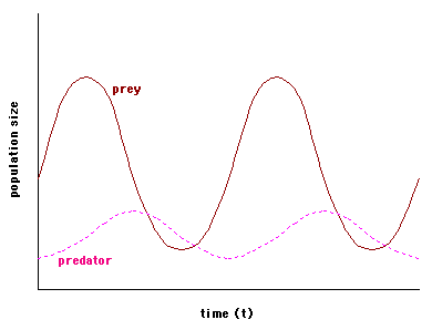
Introduction: The Lotka-Volterra model is composed of a pair of differential equations that describe predator-prey (or herbivore-plant, or parasitoid-host) dynamics in their simplest case (one predator population, one prey population). It was developed independently by Alfred Lotka and Vito Volterra in the 1920's, and is characterized by oscillations in the population size of both predator and prey, with the peak of the predator's oscillation lagging slightly behind the peak of the prey's oscillation. The model makes several simplifying assumptions: 1) the prey population will grow exponentially when the predator is absent; 2) the predator population will starve in the absence of the prey population (as opposed to switching to another type of prey); 3) predators can consume infinite quantities of prey; and 4) there is no environmental complexity (in other words, both populations are moving randomly through a homogeneous environment).
Importance: Predators and prey can influence one another's evolution. Traits that enhance a predator's ability to find and capture prey will be selected for in the predator, while traits that enhance the prey's ability to avoid being eaten will be selected for in the prey. The "goals" of these traits are not compatible, and it is the interaction of these selective pressures that influences the dynamics of the predator and prey populations. Predicting the outcome of species interactions is also of interest to biologists trying to understand how communities are structured and sustained.
Question: What are the predictions of the Lotka-Volterra model? Are they supported by empirical evidence?
Variables:
| P | number of predators or consumers |
| N | number of prey or biomass of plants |
| t | time |
| r | growth rate of prey |
| a' | searching efficiency/attack rate |
| q | predator or consumer mortality rate |
| c | predatorís or consumerís efficiency at turning food into offspring (conversion efficiency) |
Methods: We begin by looking at what happens to the predator population in the absence of prey; without food resources, their numbers are expected to decline exponentially, as described by the following equation:
![]() .
.
![]() .
.
Turning to the prey population, we would expect that without predation, the numbers of prey would increase exponentially. The following equation describes the rate of increase of the prey population with respect to time, where r is the growth rate of the prey population, and N is the abundance of the prey population:
![]() .
.
![]() .
.
Equations (2) and (4) describe predator and prey population dynamics in the presence of one another, and together make up the Lotka-Volterra predator-prey model. The model predicts a cyclical relationship between predator and prey numbers: as the number of predators (P) increases so does the consumption rate (a'PN), tending to reinforce the increase in P. Increase in consumption rate, however, has an obvious consequence-- a decrease in the number of prey (N), which in turn causes P (and therefore a'PN) to decrease. As a'PN decreases the prey population is able to recover, and N increases. Now P can increase, and the cycle begins again. This graph shows the cyclical relationship predicted by the model for hypothetical predator and prey populations.

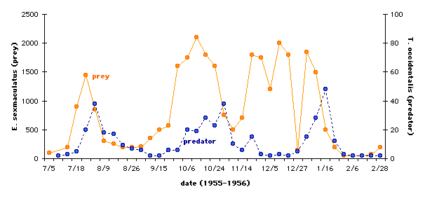
Huffaker (1958) reared two species of mites to demonstrate these coupled oscillations of predator and prey densities in the laboratory. Using Typhlodromus occidentalis as the predator and the six-spotted mite (Eotetranychus sexmaculatus) as the prey, Huffaker constructed environments composed of varying numbers of oranges (fed on by the prey) and rubber balls on trays. The oranges were partially covered with wax to control the amount of feeding area available to E. sexmaculatus, and dispersed among the rubber balls. The results of one of the many permutations of his experiments are graphed below. Note that the prey population size is on the left vertical axis and the predator population is on the right vertical axis, and that the scales of the two are different (after Huffaker, 1958 [fig.18]).

Interpretation: It is apparent from the graph that both populations showed cyclical behavior, and that the predator population generally tracked the peaks in the prey population. However, there is some information about this experiment that we need to consider before concluding that the experimental results truly support the predictions made by the Lotka-Volterra model. To achieve the results graphed here, Huffaker added considerable complexity to the environment. Food resources for E. sexmaculatus (the oranges), were spread further apart than in previous experiments, which meant that food resources for T. occidentalis (i.e., E. sexmaculatus) were also spread further apart. Additionally, the oranges were partially isolated with vaseline barriers, but the prey's ability to disperse was facilitated by the presence of upright sticks from which they could ride air currents to other parts of the environment. In other words, predator and prey were not encountering one another randomly in the environment (see assumption 4 from the Introduction).
Conclusions: A good model must be simple enough to be mathematically tractable, but complex enough to represent a system realistically. Realism is often sacrificed for simplicity, and one of the shortcomings of the Lotka-Volterra model is its reliance on unrealistic assumptions. For example, prey populations are limited by food resources and not just by predation, and no predator can consume infinite quantities of prey. Many other examples of cyclical relationships between predator and prey populations have been demonstrated in the laboratory or observed in nature, but in general these are better fit by models incorporating terms that represent carrying capacity (the maximum population size that a given environment can support) for the prey population, realistic functional responses (how a predator's consumption rate changes as prey densities change) for the predator population, and complexity in the environment.
Additional Question:
1) How would increases or decreases in any of the
parameters r, q, a', or c affect the rate of
change of either the predator or prey populations? How would the shape
of the graph change?
Sources: Begon, M., J. L. Harper, and C. R. Townsend. 1996. Ecology: Individuals, Populations, and Communities, 3rd edition. Blackwell Science Ltd. Cambridge, MA.
Gotelli, N. J. 1998. A Primer of Ecology, 2nd edition. Sinauer Associates, Inc. Sunderland, MA.
Huffaker, C. B. 1958. Experimental studies on predation: dispersion factors and predator-prey oscillations. Hilgardia 27(14):343-383.
copyright 1999, M. Beals, L. Gross, and S. Harrell